Pump system analysis: Understanding performance and system curves

Context is a useful tool for problem solving and decision making. Many of life’s decisions are arrived at only after a series of reference points are reviewed. For instance, anyone would call a 50 Euro loaf of bread unrealistically expensive, because a lifetime of bread buying tells you that it should cost much less. The same principle applies when attempting to analyse the performance of the pumping system in an industrial-manufacturing application with a liquid-handling function. When assessing pump perfor-mance and diagnosing any performance-related issues, having reference points with which to compare current performance can be an invaluable tool, resulting in a streamlined, cost-effective, durable, safe and completely optimised operation that will provide years of reliable service.

Reading pump performance curves

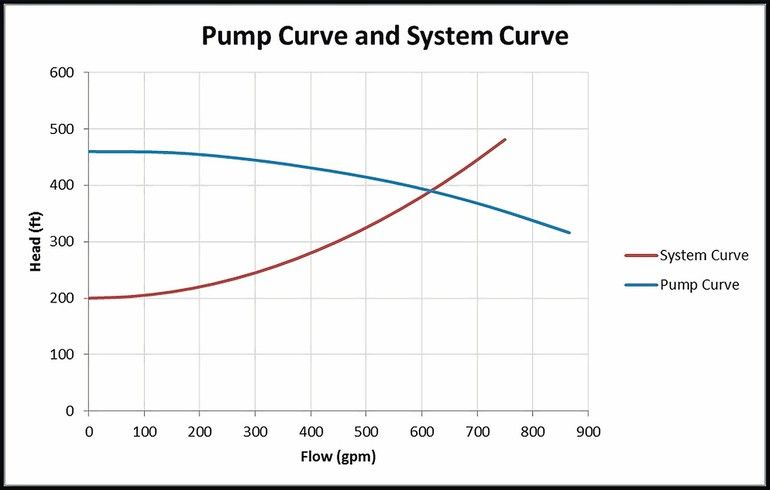
Performance curves – once you have attained the necessary context – are easy to understand and can be reliable allies when determining the limits of a pump’s operational capabilities. The first thing to know is that all pumps, no matter the operating principle, are simple machines, meaning that they don’t have a mind of their own but instead will always operate at the intersection of the pump’s performance curve and system’s resistance curve. So, because pumps operate so predictably, knowing as little as two performance curve data points provides the operator a lot of powerful information.

The published performance curve is only half the equation regarding predicted pump performance; the other half is the pump’s system curve. You should not be put off by complex performance curves, rather you should understand the system curves for calculating the performance of the pumps.

Reference values are often missing due to a lack of knowledge of pump technology. Over the years, moreover, pumps and piping may have been added or subtracted from the system. Since many alterations may occur over time, accurate system diagrams are then often no longer available, nor is the original designer. Operators must be able to overcome their initial fear of the system curve, knowing that a full understanding of the curve will have many benefits for the user:

• Improved ability to understand any future new installations and upgrades to existing setups
• A baseline for sanity checks on pump performance that compares input information to known capabilities
• Better ability to choose the best pump technology for the system’s needs
• Increased knowledge on how to select the right pump technologies to solve even long-standing problems.

Working with the system curve

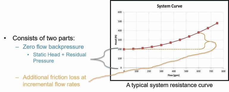
That process begins with familiarity with the system curve, which consists of two parts: flow and pressure. Every pumping system experiences flow resistance against a set flow rate. So, a basic system curve is the flow resistance plotted at fixed flow conditions. The system curve uses the same two axes as a performance curve: the X-axis is always flow rate and the Y-axis is always pressure.

There are two contributors to every system curve: friction loss and residual pressure. A system curve crosses the Y-axis at the residual pressure and slopes upward according to the friction loss. Friction loss is piping’s resistance to flow. Like increasing drag on a sports car, pipe-friction loss increases as flow velocity increases. From basic fluid dynamics, the Darcy-Weisbach equation shows a very convenient square relationship between velocity and friction loss.

Residual pressure is the system’s zero-flow backpressure. It quantifies the system’s base-level resistance at zero flow rate. It consists of two parts, net elevation difference between source and destination (i.e. static head), and residual pressure difference between source and destination.

Many sources are available to calculate friction loss, including Blackmer Bulletin 33, which tracks friction loss for all pumps and all liquids at viscosities up to 1000 cP. To create a system curve, simply calculate the friction loss at two or more flow rates, add or subtract the zero-flow backpressure and plot those points on the same pump-curve axis. Then plot subsequent intermediate points using the simple square Darcy-Weisbach relationship: half the flow, one-quarter the friction loss.

Measuring friction loss can be even easier. With two pressure gauges, you can simplify the creation and use of system curves. If you put a gauge at each of the inlet and discharge ends of the pump, the difference in the two pressure readings will indicate the differential pressure or differential head. This will enable the plant operator to quickly cross reference where the pump operates by checking the measured differential pressure or differential head against the pump curve.

Plotting system curves is especially useful for systems that operate in a variety of conditions or have a wide operating envelope. Simply plot system curves that correspond to your system’s extremes to see the full range at which the pump will operate.

Rise to shutoff

After assessing the operating range of a pump system, it’s important to check for problem zones, especially when using centrifugal pumps. Centrifugal pumps have three zones on their performance curves: shutoff, Best Efficiency Point (BEP) and runout. If a system operates near runout (or the steep portion of the curve far from the Y-axis), the motors will experience an overload current and pump reliability will decrease from cavitation. If it operates near shutoff (or the flat portion of curve near the Y-axis), the pump and surrounding components will have reliability issues, and even experience destructive water hammer.

Rise to shutoff is defined as the difference between the pump’s operating point and the shutoff pressure. For example, a 3×4-8 pump must deliver 189 l/min (50 gpm), which looks to be OK because on the system curve it is to the right of the manufacturer’s minimum recommended flow rate (MRF). But what happens if there is a slight pressure change of as little as 0.07 bar? That 0.07-bar change may appear to be negligible, but that pressure drop can create a flow-rate flux of as much as 606 l/min (160 gpm) in this example. So, a flow rate that can accumulate between 0 and 606 l/min can result in dynamic water-hammer pulses, the level of which will be further exasperated if any control devices are being used, resulting in severe pumping-system damage.

A rule of thumb for hydraulic stability is to maintain at least a 3 % rise-to-shutoff factor, though 5 to 7 % is more desirable. Anything less than 3 % will result in fluctuation issues because, again, simple pumps don’t know where they best operate because a pressure signal may be telling them they are operating effectively within a 606 l/min range.

Complex pump systems

The introduction of inline devices (filters, valves, strainers, heat exchangers, etc.) adds complexity to the pumping process. What if one of the valves is closed or a filter is clogged? You can measure friction loss where a valve is closed or a filter is clogged and then plot the new performance and system curves. If the range of system curves shows that your pump operates in a danger zone, the filter may need to be back flushed to restore proper operation. Or it may indicate a need to maintain tank levels to facilitate a smooth, efficient pumping process.

Another variable is multiple flow paths in the pumping process. Examples of this include closed cooling-water systems and burner systems, when one pump feeds multiple users. In setups like these, the overriding question is: which flow path to use to analyse the pump’s performance and system curves? It doesn’t matter. Like an electrical circuit, the parallel paths in a closed-loop system balance, with any friction loss the same in all parallel paths. Size the pump for the loop with the highest back pressure and the balancing valves will simulate equal back pressure for the other flow paths.

Blackmer, Grand Rapids, USA